Espresso Simulation: First Steps in Computer Models
Espresso is a reaction of coffee, pressure, and hot water. We can observe the preparation, the bottom of the filter, and taste/measure the resulting espresso. However, we can’t see inside the shot. Some work has been done to make transparent portafilters, but they only give a view from the side.
What really goes on inside the espresso shot?
I started an effort to understand how to simulate an espresso shot six months ago because a simulation could allow you to see a cross-section view and potentially understand and model different properties leading to improvements in real shots. The key was making a realistic model usually through trial and error to make sure the mode matches observation. Here is the list of factors I wanted to model prioritized in order (to go from a simple model to a more complex model):
- Grind size
- Grind distribution
- Filter hole size/distribution
- Shower screen hole size/distribution
- Water flow
- Dynamic changes inside the puck as coffee is extracted
For this first simulation, I focused on the top three in a static fashion (not accounting for the coffee grounds changing as extraction occurs). I quickly ran into some trouble, but the journey is very important.
First Model: Horizontal Cross-Section
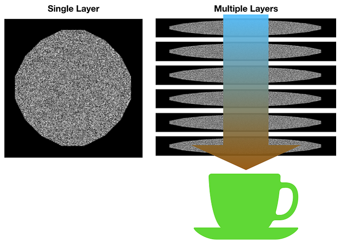
The first model I had designed would use horizontal cross-sections of the coffee puck, and I would stack these cross-sections on top of each other. Each cross section would have holes for water to flow through. I wanted to use morphological operations to estimate the grounds shrinking as the coffee is extracted. However, there was difficulty in connecting layers, and I decided to rethink it.
Second Model: Vertical Cross-Section
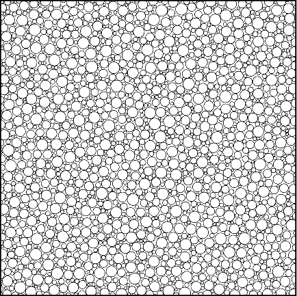
Instead of horizontal cuts, I thought trying a single, vertical cross-section might work better. I started trying to figure out how to draw the circles to represent the grounds. I found a function that could draw circles given some distribution, but the difficulty was how to model the shot overtime. As the water goes through, coffee is extracted, but if you make the circles smaller, does that really map to how the coffee is being extracted or the flow through the area? Shouldn’t the circles compact down on one another?
Additionally, how large of an image does one have to make to get the desired resolution? For fine particles, they are 100 um in diameter. If they shrink by 30%, that’s 70 um. So at the least you need 10um resolution or even 1 um. However, at 10 um resolution for a 58 mm diameter and 20 mm depth, the image would have to be 5,800 x 2,000. For 1 um, that would be 58,000 x 20,000.
The other challenge was re-generating this image for every cycle. Using the function Bubblebath, random circles could be drawn. The function needed modification to get similar coffee particle size distributions, and I became convinced a better way would be had than using this function on a 11 megapixel image. This image below took a minute to generate, which is fine for a single static plane, but not when looking at an ever changing plane over time.
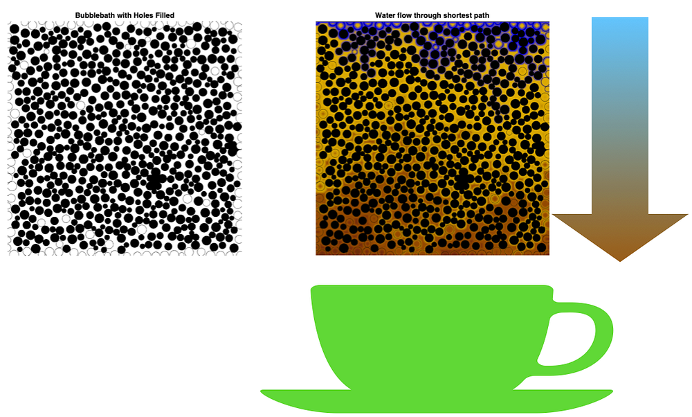
Here is how water would flow for this model. One can see some of the channeling inside the shot simply due to the randomness of the circle sizes and distribution.
Third Model: Vertical Cross-Section in Grayscale
Back to the drawing board, I thought more about quantizing the coffee puck. Using an 11 megapixel image or anything near that size would make development time for the model long without providing as much benefit. Once the model was developed, you could increase the size, so quick development time became the priority.
What if every pixel represented the density of particles at that location?
If every pixel was a density of coffee for that location, determining how water flows is the minimum path from the shower screen to the filter screen. To determine how the puck changes due to extraction, that minimum path can be used to modify the intensity of each pixel over time as the densities and paths change.
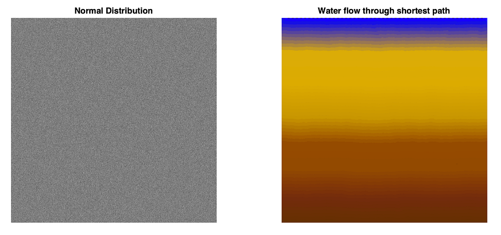
This method is also easier to have a separate color plane to represent the water and what’s being dissolved in the water. My focus for this initial study was to find a method where I could view the cross-section over time.
When just examining the shortest path, we can see some of the channeling issues before the shot is pulled. As the shot is pulled, it will change the densities around the puck. There is this initial assumption that evenly distributed pucks shouldn’t have channeling. With this model, I’ve found channeling occurs no matter how Gaussian the grounds are distributed. This means that even the best distributed pucks will have channeling.
How much channeling is acceptable?
Another point to consider is that even with a bottomless portafilter, you are unable to observe anything other than major channeling or major channeling that isn’t underneath the main flow of the shot. Only a more advanced sampling of the shot would allow one to see the full puck.
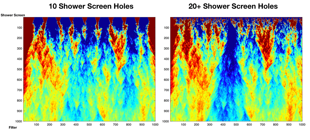
Back to the model, let’s see how shower screens could effect flow. Below is looking at the same puck in terms of grounds distributions or densities, but with 10 or 20 shower screen holes. The graph itself is colored based on each row using the jet color scheme: red shows slower flow, and blue shows faster flow relative to the current row, and the transition from red to orange to yellow to green to blue show the variations.
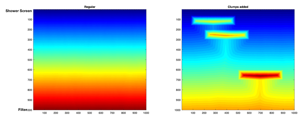
I’ve added spots for really dense areas to simulate chunks that where broken up. This shows the flow as the shortest path to each point from the top. The clumps end up causing the water to go around them, so the more clumps there are, the less extraction that’s occurring. This picture shows the globally normalized flow rather than row normalized.
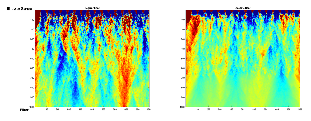
Another interesting piece is modeling different distributions for staccato shots. The layers have a tighter size distribution, but even the mid layer at the top has issues. The mid layer should have the tightest distribution of all the layers but there’s still channeling. Same with the coarse layer. It seems the fine layer helps smooth some of the channeling at the end.

It’s pretty straight forward to compare flow for regular vs staccato, but they will be inherently different distributions. Even the colorization needs modified because you can’t see the finer differences in the staccato shot in the bottom layer. There are flow differences, but they are on a smaller scale.
Originally, I wanted to wait before I made more insights, but even the model design has been tricky. At the moment, this seems to be the right direction, but there may be a better way to model these complexities. By exposing the thought process and iterative design of the model, I hope to inspire others to do the same. I hope that through simulation along with real world measurements, we’re able to find major improvements and understandings to how to brew espresso.
If you like, follow me on Twitter and YouTube where I post videos of espresso shots on different machines and espresso related stuff. You can also find me on LinkedIn.
Further readings of mine:
Staccato Espresso: Leveling Up Espresso
Coffee Solubility in Espresso: An Initial Study
The Tale of the Stolen Espresso Machine
Affordable Coffee Grinders: a Comparison
